How to Format Number as Currency in Excel
Excel users wanting to display numbers as monetary values, must first format those numbers as currency. To do this, apply either the Currency or Accounting number format to the cells that you want to format. The number formatting options are visible under the Home tab of the ribbon menu, in the Number group.
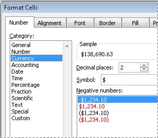
Next, for displaying a number with the default currency symbol adjacent to it, select the cell or range of cells, and then click Accounting Number Format Button image in the Number group on the Home tab. (If you want to apply the Currency format instead, select the cells, and press Ctrl+Shift+$.) If you would like to change other aspects of formatting for your selection, Select the cells you would want to format. Next, on the Home tab, click the Dialog Box Launcher adjacent to Number. See the screenshot below. Then, in the Format Cells dialog box, in the Category list, click Currency or Accounting.
Thereafter, under the Symbol box, click the currency symbol that you want. If you do not wish to display a monetary value, simply choose the None option. If required, enter the number of decimal places that you want for the number. As you make changes, it will reflect in the number in the Sample box, indicating changing the decimal places affect the display of a number. Now read: How to perform calculations with Range Calculations app for Excel.


